Co-authors: Ying Jin, Shiqing Li, Xiao Li

This post we present the attempt to solve a novel problem of estimating the surrounding bird eye layout of a complex driving scenario with six different camera perspective images only. While existing literature aims to approach this set of problem with a pre-trained neural network with ability to detect object given images, and rely on intrinsic and extrinsic calibration data to transform from perspective view(s) to bird eye view (BEV), we followed the idea from MonoLayout to derive a single model that transform from perspective view to BEV and segments objects all-in-one. We also propose an architecture using both ResNet and U-Net that outperforms the MonoLayout architecture.

Introduction

This work performs an interesting and highly challenging task of constructing a road map and identifying locations of the surrounding objects at the same time using color photos of six different directions taken from a car on the road.

While most research treat generating road map and object bounding box as separate tasks, we are inspired by the idea from MonoLayout which argues that roadmap task and object detection task should be trained together as they are highly correlated since objects are moving on the road. We further improves MonoLayout’s architecture by using a shared encoder with ResNet backbone and two U-Nets with the same structure to decode bird eye view (BEV) maps. Both BEV road map and objects are predicted as binary square matrices. Post processing were done on the object maps to generate bounding box coordinates.

Since the labeled data is rather limited, utilizing the unlabeled data adequately is an important factor for us to improve our model’s performance. We adopted the method from Monodepth2 to conduct self-supervised learning on both labeled and unlabeled dataset to extract depth information from every image.

MonoLayout’s idea of infusing patch-level discriminators is also adopted in our work to close the gap between generated output distribution and ground truth layout distribution.

Results show that the shared encoder and our proposed network effectively improves the prediction compared to training individually or using MonoLayout’s architecture.

Method

Data Description

The data set contains 134 scenes, each with 126 samples that make up a 25 second journey. 28 of the 134 scenes are labeled, with 22 random scenes in training and 6 in validation set.

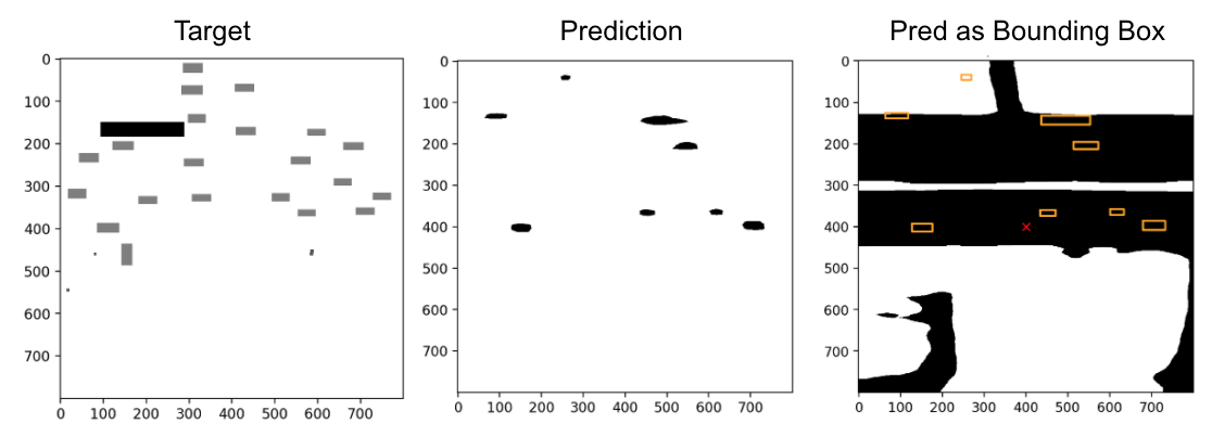
In this work, each sample’s corresponding bounding box coordinates are preprocessed to be an object matrix, same size with the road map, where the value corresponds to different object types. In this work, we further reduced the problem to made binary prediction of object vs. non-object. The bounding box coordinates for objects are identified using skimage by boxing clusters of positive prediction on the object map matrix. Figure 1 shows an example of target, prediction, and its final bounding box result. Note that the current pre and post processing steps are naive in that they assume objects are parallel to the axes.

All images, with or without labels, are used to learn depth in a self-supervised network. The depth is used to enrich the input as an added feature.

Model Architecture

HexaLayout Architecture

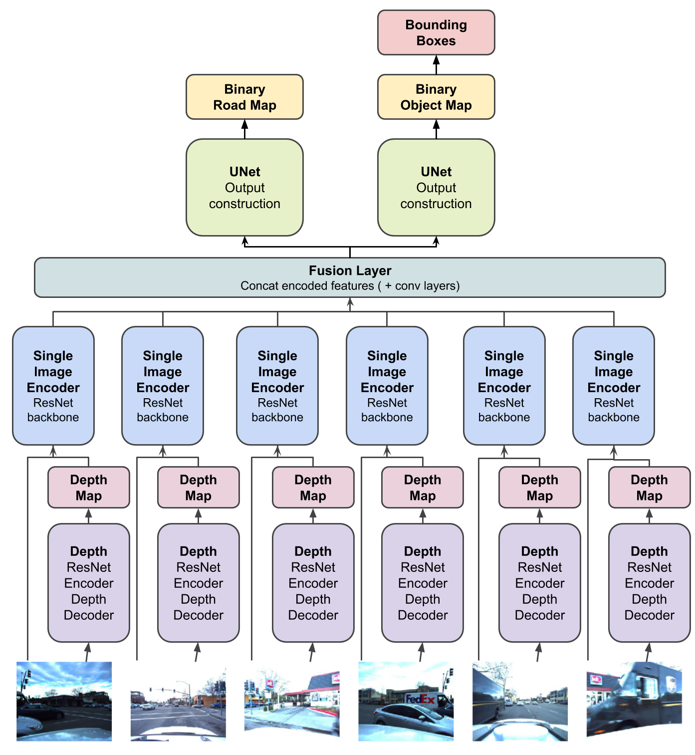
The base architecture for HexaLayout is shown in the top part of figure 2. The model, implemented using PyTorch, consists of six shared weight single image encoders using three-block ResNet with filter sizes [64, 128, 256]. In the fusion layer, six encoded features maps are concatenated along feature map dimension based on each camera’s respective location in reality. The outputs are fed into two U-Nets with the same structure and separate weights to construct final predictions. Both outputs are interpolated to 800 * 800 to measure loss against original road and object maps. Model weights are trained using combined loss from road and object map losses.

We improved upon MonoLayout encoder decoder architecture by using a shallow ResNet encoder without dense layer and a U-Net to reconstruct the outputs. Removing dense layer in the encoder allows the feature maps to localize the spatial location of each encoded features. Using U-Nets that have shortcut connections from encoder to decoder helps carry encoded features forward to the final layers. These modifications improve the prediction results as shown in Result section.

Model Variations

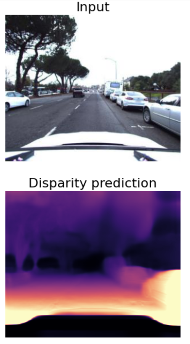
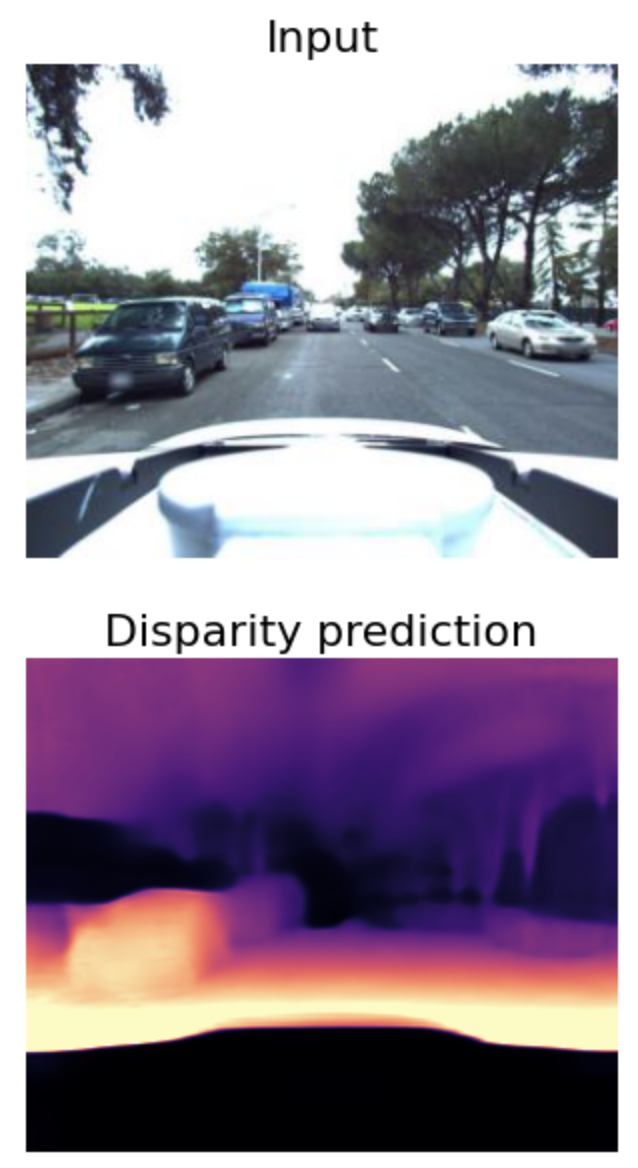
Adding depth information We believe depth information is helpful for our model to learn a top-down bird’s eye view from perspective images. Hence we adapt the method of Monodepth2 to perform a self-supervised learning task on our dataset to obtain the depth information from raw images. The Monodepth2 model uses 3 consecutive frames of monocular images and tries to minimize the reprojection error between the reconstructed image and the target image (frame 0) where the reconstructed image is constructed by using the pose information obtained from estimating the relative pose between the target image and one of the other source images (frame -1 or frame 1) and the depth information which is obtained by passing the target image to a U-Net depth network. We trained 6 depth models, each for one specific camera perspective. Figure 3. shows some examples of our depth models’ outputs.

We tested 3 variations from HexaLayout, 2 of them utilizes depth information and the last one uses discriminator:

Variation 1: Depth as Input The first is shown in Figure 2. by adding the depth maps as the 4th channel of the raw input images and then pass these 4 channel image matrices to the encoders.

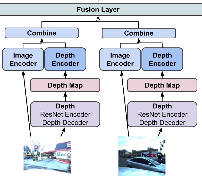
Variation 2: Encoded Depth Feature The second is illustrated in Figure 4. by passing the depth maps to a separate set of encoders which share the same architecture as the single image encoders but with different weights, then concatenate the encoded feature maps with image encoder outputs along channel dimension and pass to the U-Nets.

Variation 3: The Discriminator The discriminator network is adapted by PatchGAN to encourage high-frequencies detection and low-frequency correction, otherwise network would easily led to blurry results if not carefully trained. The architecture allows the discriminator to classify each N x N patch of an image whether it is provided in training set (real) or model generated (fake). Both outputs generated by the road map and object decoder are feed into two separate discriminators. By comparing to the ground truth output distribution in BEV, the gap between predicted output layout and ground truth output layout should be minimized along training.

Loss Function

Since both road map and object map predictions are reduced to tasks of binary map prediction, we tried both nn.BCEWithLogitsLoss() with final layer feature size = 1 and nn.CrossEntropyLoss() with final layer feature size = 2. The results are comparable. The discriminator also utilizes BCE loss as it feeds by a confidence score distinguishing real or fake output distributions.

Results

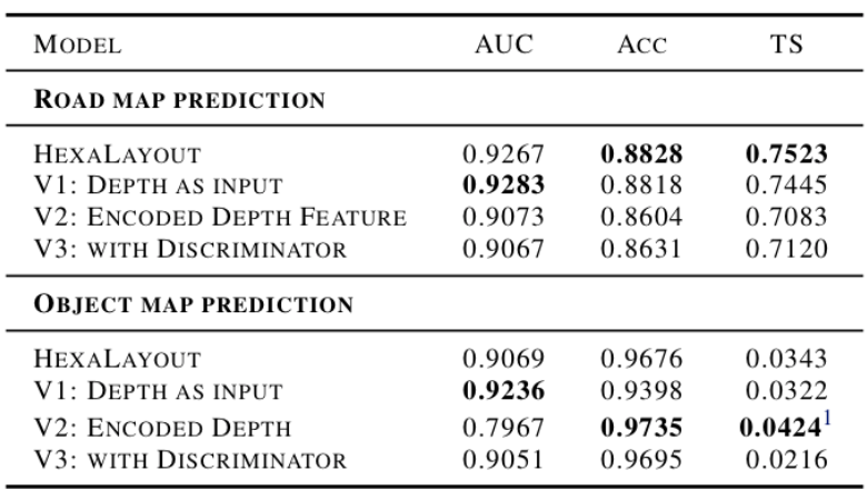
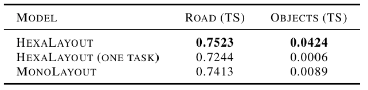
Mean area under the curve (AUC), accuracy (Acc), and threat score (TS) are measured pixel by pixel for road map prediction. We also measured AUC and Acc for object map on a pixel by pixel basis. Average mean threat score are measured for the final bounding box prediction as instructed, at different intersection over union (IoU) thresholds [0.5, 0.6, 0.7, 0.8, 0.9]. Validation results for HexaLayout and three of its variations are shown in Table~\ref{model_results}.

Table~\ref{model_encoder} demonstrates that the shared encoder improves the prediction threat score, especially drastically for object map predictions. In addition, our proposed network outperforms MonoLayout’s architecture on the object detection task by a significant margin.

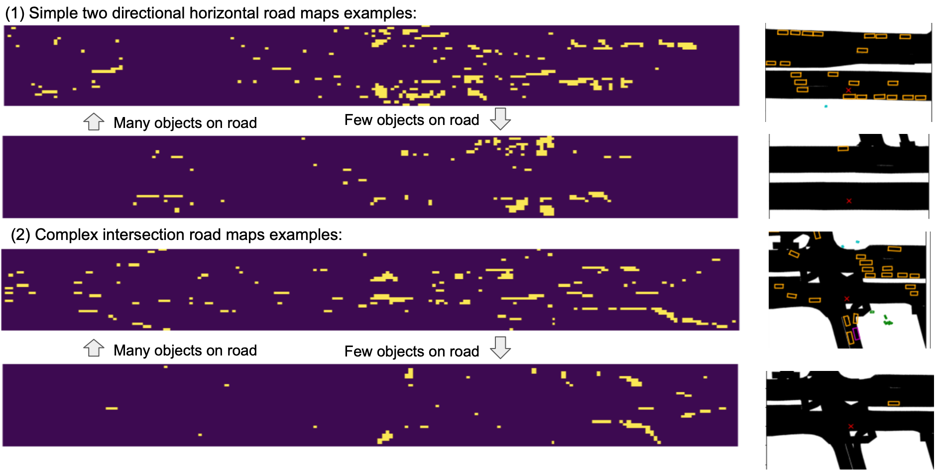
Encoded Features To understand our model’s learning capacity, features maps are visualized to see if the model recognizes specific patterns of inputs. By selecting and concatenating 4 out of 256 feature maps from ResNet encoder output, the neurons can be observed to be activated at specific locations with different sample inputs. Results from 4 samples are shown in Figure 5 to demonstrate model interpretability. Fewer neurons are activated when there are few objects on the road; further, neurons seem to activate at different locations with different road map structure.

Prediction Analysis Further analysis done on the prediction results exposes weakness of the current architecture and suggests ideas for future research directions.

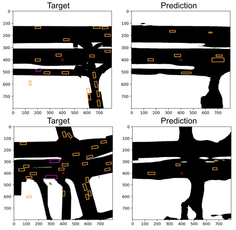
Figure 6 shows that the object map predictor preforms better for objects that are closer to the ego car, which is expected since objects further away are often blocked by an object that’s closer. We believe that adding an additional one directional temporal module could expose the model to context on previous time steps, therefore, potentially improving prediction on objects further away.

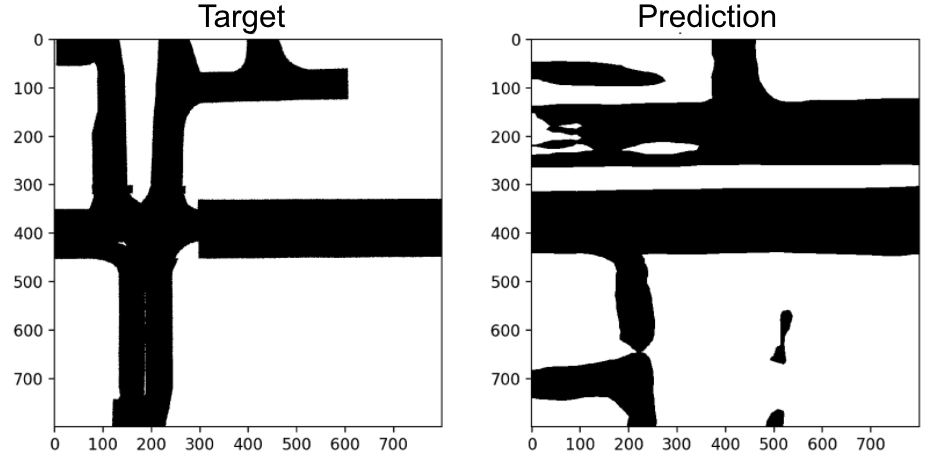
We also found that, since most of the training examples contains two horizontal lanes and sometimes one vertical lane, the model almost always predicts two horizontal lanes and, if there is a vertical lane, the prediction would contain only one. In Figure 7, the model made patchy predictions for the top horizontal lane, meaning it identifies the distinction but fails to realize that this sample has one lane only. Feeding the model with more of those unique samples should help with this issue.

Another direction for future work would be to use pre-trained weights for the ResNet encoder, allowing the model to identify objects more accurately.