Co-authors: Cody Fizette, Ying Jin, Shiqing Li

Data and Model Overview

In this post, we presernt a recommender system that is a collaborative filtering model attempting to recommend fresh songs to users based on the songs they listened to previously. The training dataset consists of 50,000,000 data points. Each data point contains a user_id, a track_id, and count. In total, there were approximately 1.1 million users and 385,000 songs. Count is seen as an implicit feedback (the number of times the user listened to the song). The type of feedback affects how we built the recommender system as will be discussed in the following sections.

Collaborative filtering is a method widely adapted for recommender systems. This method defines similar songs not because they are of the same type or written by the same musician, but because they are consumed by the same group of users, assuming that users who agree in the past would tend to agree in the future. The interaction matrix is often in high dimension and sparse. Matrix factorization effectively brokes the interaction matrix (rating matrix) down into a product of two lower dimension matrices, the user and item matrix. The rank of the user and item matrix correspond to the number of latent factors. The model tends to overfit with high latent factors (rank). The objective is to minimize the error between true ratings and predicted ratings.

In this work, we used Alternating Least Square (ALS) to solve the collaborative filtering problem. ALS is suitable for large scale problems as it runs in a parallel fashion across multiple partitions. It minimizes the loss function for user matrix and item matrix alternatively. In each round, it holds one matrix and runs gradient descent on the other. In addition, the objective function is regularized using L2 regularization.

Our work employs the ALS implementation in PySpark. Using both grid search and random search, we fine-tuned hyperparamters including rank (number of latent factors), regParam (l2 regularization parameter) and alpha (the scaling parameter for implicit feedback).

Evaluation Metrics

Our goal of this work is to recommend a short lists of items that match user’s preference. We aim to take each item’s rank into account, such that users can easily discover items matching their favor on the top of recommended lists.

Precision at K, P(k) uses an indicator function that returns 1 if the jth recommended item from Ri for user i is found in the true preference list Li. And k truncates the range of examination to the top k recommended items. Precision at K is not an ideal metric since it does not consider the actual rank from a recommender system.

Mean Average Precision (MAP) uses the same indicator function adopted from Precision at K, also returns an average score among all users. Different from Precision at K, MAP examines entire Ri for each user, but predicting a correct item with a higher rank in each Ri will receive a higher score.

Normalized Discounted Cumulative Gain (NDCG) at K considers rank similar to MAP, while it only evaluates the top K items from Risimilar to Precision at K. Since the order of the list was important to evaluate the recommender system, we choose MAP of the first 500 evaluate model performance, although NDCG at K also considers rank, the penalty term is logged and thus it is not as sensitive as MAP.

Model Implementation details

Our model is built in PySpark using DataFrame based ALS module, and the outputted ranking is evaluated using the RDD based RankingMetrics module. The ALS module gives two ways of generating predictions on validation and testing data sets. One through the recommendForUserSubset(users, k) method, which returns top k predicted items and their corresponding ratings for each user. The other is through the transform(validation_dataset) method, which generates a probability for each of the user/item pair. Through experiments we found that the transform() do not touch every single items since it only returns score for items that are included in the validation dataset, therefore yielding a MAP of 1 every time. To adhere to the goal of this project, we decided to use the recommendForUserSubset() method.

Note that we are evaluating on the validation dataset along, in which the validation items for a given user is different from those in the training dataset. The recommender system should successfully suggest new items that correspond to each user’s preference implicitly received from their viewing history. We believe that evaluating on this new set of items, as opposed to the combination of train and validation, makes the most sense, since in our application it is not desired to recommend items that users consumed in the past.

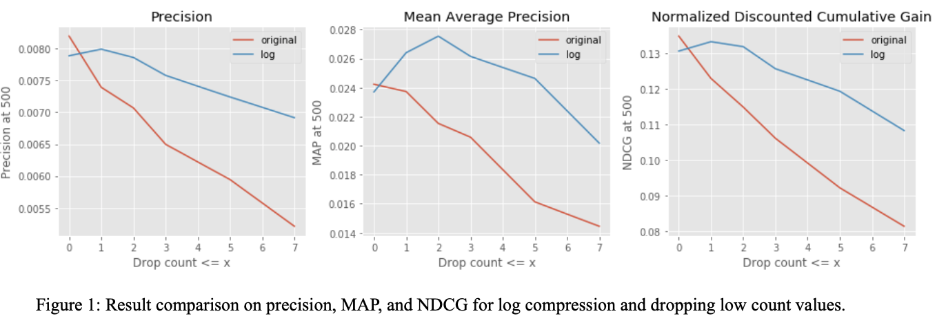
With guidelines from the work in Hu et al., 2008, we experimented searching the best hyperparameters using both random and grid search on the following range: rank [5, 500], regParam [10e-5. 10e3], alpha [1, 25], model performance is shown in Fig 1.

Extension: Alternative model formulations

Since count is considered as an implicit feedback, and implicit feedback may not accurately represent user’s preference because it has inherent noise and we assume there is a positive correlation of count value with user preference. Second, count in our dataset is skewed, as there are large extreme counts up to 140, while the average count is ~2.5.

We approached to take the log of count to compress extreme values. Nearly 60% of data has a count of 1, transforming count by logging with offsetting avoid compressing count of 1 to 0. From figure 1, we observe that after applying log compression on our unfiltered dataset, the performance decreased. However, with log compression and data filter applied together, MAP reached an optimum that is ~14% higher after dropping count<=2, though the performance decreased as we increase the dropping threshold. With log compression and drop count <=2, we arrived at the best performance on valuation set with MAP = 0.004586 shown in Fig 1.